

In an earlier article, we explored use case for soft sensors and made one for MFR and density prediction in gas phase alpha-olefin polymerization. Using simple models, we were able to get relatively good dynamic predictions when applied to real trajectories.
Unfortunately, we also saw that when MFR was around 2.0, the cumulative property prediction showed the largest offset when compared to lab measurements. My previous claim was that it is still possible to use the models effectively where they actually matter - such as when used in process control; to bridge the model error gap, we have to somehow make use of the intermitten lab feedback.
Internal Model Control
Internal Model Control (IMC) is a powerful control law that naturally combines feedforward action with feedback action. It is easy to implement and tune, and can be used to derive optimal PID controller tunings without invasive step tests.

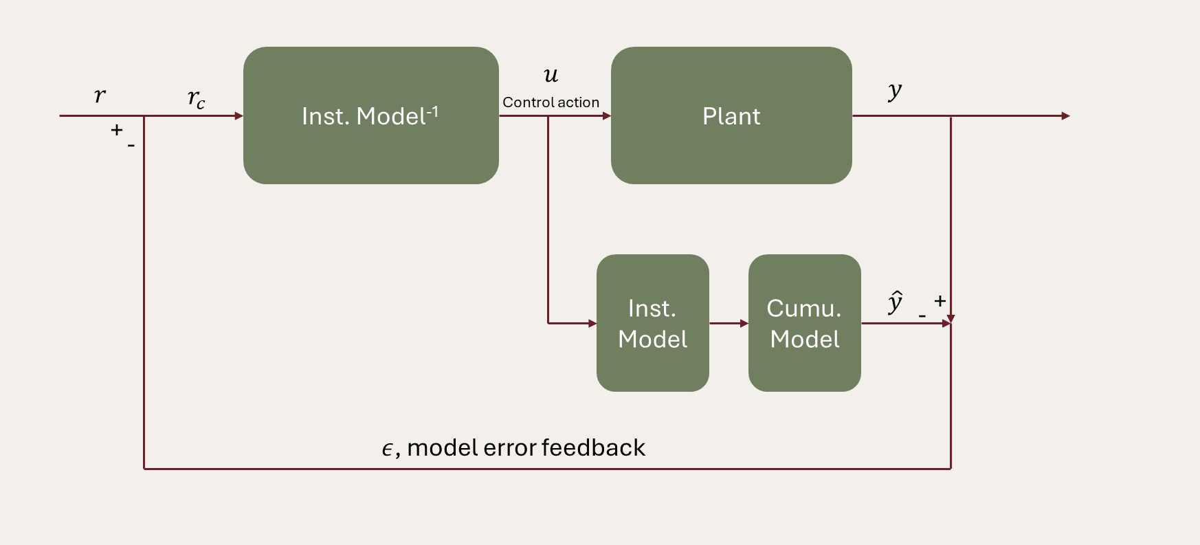
r is the reference, or setpoint, we are trying to control y, the process variable, to. Since lab results take time (typically around 1 hour for MFR and 4 hours for density), it necessitates a modified block diagram where the plant feedback is discrete and backwards looking instead of continuous. The feedback law then becomes
Importantly, the lab times are *sampling* times, not result reading time.
Typically, the IMC controller is derived by inverting the model and applying a filter. The filter is tuned to describe the desired closed loop response. In (simplified) transfer function talk, the control law looks like.
g_c is the control transfer function, f is the filter, and g_m is the model transfer function. If the model is perfect (i.e., g_m=g_p, where g_p is the process transfer function), then the closed loop plant transfer function simplifies to the chosen filter f(s).
All this is to say, in the ideal world, we can pick the desired response shape and implement that as the filter; the simplest case is a first order filter with some time constant \tau_{CL}.
In our case, we will actually pick an unusual filter of... 1! Because the instantaneous properties are already filtered at the reactor bed open loop time constant (the residence time) to calculate the cumulative property (which is the thing we want to control), we do not need to worry about unphysical transfer function and control actions that are typically associated with such IMC filters.
The resulting control block diagram for our system then looks like this below, where the controller block is replaced with the inverse of the instantaneous model.
Enough theory, lets see it in action for some transitions.
IMC Control Performance
Below shows 2 transitions - one large MFR increase with no density move, and one where both MFR and density increases.

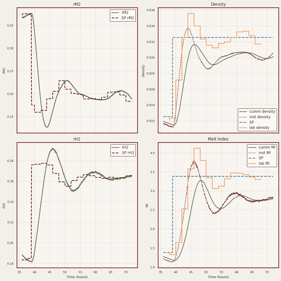
As promised, despite significant model offset in both MFR and density (and my terrible composition control tuning...), both properties converged under closed loop control, as shown by the lab results converging around the dotted-blue property setpoints.
Unexpected Control Moves
One interesting observation from the first transition where density stayed constant: significant comonomer molar ratio rM2 move was necessary to keep the density from drifting as MFR started changing.
Recall that in the correlation heatmap from our exploratory data analysis, neither rH2 nor MFI target had significant correlation with density, yet our observation from closed loop control seems to suggest otherwise. This is a great example of the iterative nature of soft sensor development and deployment.

Conclusion
In this blog, we explored a simple way of deploying soft sensors for process control. We also showed that, despite significant model offset, convergence can be achieved with the proper application of control theory.
We also took note that either MFR or hydrogen molar ratio have significant effect on resin density. In a future blog, we will explore how to incorporate our findings to improve the soft sensor, and look into more sophisticated methods of model based/predictive control.